
Human Population Genetics and Genomics ISSN 2770-5005
Human Population Genetics and Genomics 2026;6(2):0005 | https://doi.org/10.47248/hpgg2606020005
Original Research Open Access
Selection scans and downstream analysis with selscan
Amatur Rahman
†

 ,
T. Quinn Smith
†
,
Zachary A. Szpiech
,
T. Quinn Smith
†
,
Zachary A. Szpiech
Correspondence: Amatur Rahman; Zachary A. Szpiech
Academic Editor(s): Joshua Akey, Carina Schlebusch, Torsten Günther
Received: Oct 10, 2025 | Accepted: Feb 21, 2026 | Published: Mar 20, 2026
© 2026 by the author(s). This is an Open Access article distributed under the Creative Commons License Attribution 4.0 International (CC BY 4.0) license, which permits unrestricted use, distribution, and reproduction in any medium or format, provided the original work is correctly credited.
Cite this article: Rahman A, Smith TQ, Szpiech ZA. Selection scans and downstream analysis with selscan. Hum Popul Genet Genom. 2026;6(2):0005. https://doi.org/10.47248/hpgg2606020005
Summary statistics based on Extended Haplotype Homozygosity (EHH) are widely used for inferring positive selection in genomes as a result of their ease of use, computational efficiency, and interpretability. These various summary statistics can be applied to single populations or to pairs of populations, can be used with a genetic recombination map or without, and can be applied to phased or unphased data. Although these statistics are straightforward to compute, there lacks clear descriptions on how they relate to one another, how they should be used, and how their resulting outputs should be interpreted. Here, we provide a comprehensive introduction to selection statistics as they are implemented in the widely used software,
selection statistics, extended haplotype homozygosity, positive selection, selscan
Among evolutionary biologists, there is great interest in identifying the genomic basis of adaptations. Pinpointing putatively adaptive mutations, especially in relation to known selective pressures and with functional validation, can provide insights into the biological mechanisms underlying phenotypic innovations. In humans, understanding the biological basis of adaptation can give a deeper understanding of our evolutionary history and can reveal important information about the relationship between genes, adaptation, and disease [1–3].
Given this importance, many statistics have been developed to make inferences about positive selection in the genome across different time scales [4, 5]. For detecting recent and strong positive selection, common methodologies typically make use of expected distortions in either the site frequency spectrum or haplotype patterns [6]. When a strongly adaptive allele arises, it will sweep to high frequency on a timescale faster than recombination or mutation occur, bringing linked variation to high frequency as well. This results in a region of low genetic diversity, long haplotypes, and an excess of high and low frequency alleles. Although more complicated model-based [7–13] and machine learning [14–17] methods have proven useful, especially for inferring specific parameters of a sweep, summary-statistic-based methods remain widely used as a result of their ease of use, computational efficiency, and interpretability.
One particularly important class of summary statistics for inferring positive selection are those based on extended haplotype homozygosity [18], which are designed to capture the signal of long high frequency haplotypes in the vicinity of a sweep that is either ongoing or recently completed. EHH-based summary statistics include iHS [19], nSL [20], XP-EHH [21], and XP-nSL [22], and although originally formulated for use on phased haplotype data, they have also been extended to work on unphased data as well [23, 24]. These statistics are also frequently included as important components in more advanced machine learning approaches [16, 17]. Given their broad adoption for use in selection inference analyses, they have been implemented in several widely used software programs including
In this work, we introduce the definitions of these common EHH-based statistics and their interpretations. We also provide an overview of how to use
First, we introduce the main statistics (Sections 2.1, 2.2, 2.3, and 2.4) and provide the exact commands used on simulated data. These commands match those used to produce the figures and results in the Results section, aiming to provide a quick start for users interested in performing selection scan analyses. We also highlight the importance of downstream analysis and present both its application and the relevant commands (Section 2.5). We describe our simulations and dataset preprocessing methods in Section 2.7.
Extended Haplotype Homozygosity (EHH) is the probability that two chromosomes randomly chosen from those carrying a particular “core” allele at a given locus are identical by descent across all markers from that core locus to another position [18]. Consider a sample of n chromosomes. Define
EHH between x0 and x1 of the entire sample [18, 25] is calculated as
where nh is the number of observed haplotypes of type
It is advantageous to calculate the haplotype homozygosity of a sub-sample of chromosomes all carrying a ‘core’ allele at locus x0. Define
Finally, define EHH of haplotypes containing the core allele, c, to a locus xi as
where nh is the number of chromosomes with haplotype
EHH can be adapted to unphased genotypes of diploid individuals by encoding each locus with the number of observed derived alleles: 0, 1, 2 corresponding to homozygous ancestral, heterozygous, and homozygous derived, respectively. Let
Similarly, the above reasoning can be applied when defining EHH for a ‘core’ allele. To compute the EHH of a subset of observed haplotypes that all contain the same ‘core’ genotype, let
Finally, define cEHH as the complement EHH of a sample of haplotypes. cEHH is the EHH of all haplotypes without the ‘core’ genotype at x0.
where
EHH measures the decay of haplotype homozygosity in iteratively larger windows extending from a core locus. It is computed from among all haplotypes in the sample (Equation 1) or from among only haplotypes containing a particular core allele (Equation 3). Under neutrality, haplotype homozygosity is expected to decay quickly as the window grows larger—reflecting the underlying diversity of the haplotypes in the sample. However, haplotype homozygosity will be maintained at high levels in the vicinity of a recent or ongoing sweep. In this case, EHH of all samples (Equation 1) is expected to decay slowly as window size increases, as the sweeping haplotype will dominate the homozygosity calculation. If computing EHH from among only haplotypes containing a particular core allele (Equation 3), the expected pattern depends on whether the core allele is (or is linked to) the adaptive allele. When the core allele is (or is linked to) the adaptive allele, EHH computed from among only the sweeping haplotypes will have a slow decay as window size increases. On the other hand, the EHH computed from among only non-sweeping haplotypes will have a fast decay as window size increases, similar to the expectation under neutrality. See Section 3.1.2 for an illustration.
To calculate EHH at a marker rs1 on phased data:
Assuming the input VCF file contains one chromosome, we can calculate EHH at a specific position. For example, at 5MB:
Suppose we have a file with a list of three sites, genetic.map:


Then, to run EHH at each of the three loci:
To run on unphased data, we add the
The decay of haplotype homozygosity tracked by EHH and EHHc provides useful biological information for identifying sweeps at individual loci of interest, but these statistics are not well-suited for genome-wide scans. This motivated the development of iHS, which uses Equation 3 to summarize the decay of ancestral and derived haplotype homozygosity into a single score. iHS is calculated at a site by first calculating the integrated haplotype homozygosity (iHH) for the ancestral (0) and derived (1) haplotypes (
This ensures that when the derived allele is under selection and iHH1 > iHH0, the ratio exceeds 1, the log is positive, reflecting the typical case where a positive statistic indicates selection on the derived allele. Note, this definition is different from that in [19], where the roles of iHH1 and iHH0 are swapped and a natural logarithm is used.
A related statistic, nSL, was introduced by [20]. Although Ferrer-Admetlla et al. define nSL in terms of the mean number of sites shared among all pairwise haplotypes in the vicinity of a query site, they also prove a reformulation in terms of haplotype homozygosity. Using Equation 5 above, the essential difference between nSL and iHS is that the distance function for nSL is given by g(xi, xj) = |j − i|, which simply counts the number of observed segregating sites between xi and xj.
iHS and nSL can be adapted to unphased genotypes by using the definitions in Section 2.1.2 and defining the homozygous ancestral and the homozygous derived genotypes as c = 0 and c = 2, respectively. The integrated haplotype homozygosity (iHH) can be calculated for each genotype using Equation 5, and the complement integrated haplotype homozygosity (ciHH) can be calculated for both homozygous core genotypes as
where g(xi−1, xi) is the genetic or physical distance between two loci.
The unstandardized unphased iHS is calculated as
where iHS2 = log((iHH2)/(ciHH2)) and iHS0 = log((iHH0)/(ciHH0)). Unstandardized unphased nSL is computed similarly but with g(xi, xj) = |j − i|.
iHS/nSL are intended to efficiently contrast the decay of haplotype homozygosity computed from among haplotypes containing the ancestral and derived alleles at a locus of interest. From Equation 6, when the log-ratio takes an extreme positive value, this suggests haplotypes carrying the derived allele are unusually long and low-diversity compared to haplotypes carrying the ancestral allele. When the log-ratio takes an extreme negative value, this suggests haplotypes carrying the ancestral allele are unusually long and low-diversity compared to haplotypes carrying the derived allele. It is tempting, in this case, to think that only extreme positive values are of interest, assuming that an adaptive allele is necessarily derived. However, ancestral alleles in linkage disequilibrium with the adaptive allele also provide information in the vicinity of a sweep, and in some data sets the adaptive allele may not even be observed. Therefore analyses using iHS and nSL are typically concerned with extreme absolute scores. See Section 3.1.2 for an illustration.
To calculate iHS on phased data,
To calculate iHS on unphased data, add the
When a genetic map is unavailable for iHS, the
To calculate nSL on phased data,
To calculate nSL on unphased data, add the
XPEHH [21] and XPnSL [22] were introduced as two-population extensions to iHS and nSL, respectively, intended to identify local adaptation. For these statistics, instead of comparing the EHH between haplotypes with the ancestral and derived alleles (i.e., by computing EHHc for each allele type), they compare the EHH of all haplotypes in one population to another population. Consider two populations, A and B, and a locus x0. First, iHH is calculated for each population by integrating the EHH of all samples (Equation 1) in each population.
Let iHHA and iHHB be the iHH for populations A and B, respectively. Then the unstandardized XPEHH is
XPnSL is calculated similarly, but with g(xi−1, xi) = |j − i|.
Unphased XPEHH and XPnSL can be calculated using the unphased definitions given in Section 2.1.2 and Equation 10, which defines unphased iHH for the entire population. The distance measure is either centimorgans or base pairs for XPEHH [21], or the number of observed sites for XPnSL [22]. Both XP statistics between population A and B are computed as
XPEHH/XPnSL are intended to efficiently contrast the decay of haplotype homozygosity of a sample of haplotypes from one population to a sample of haplotypes from a closely related population at a locus of interest. From Equation 11, when the log-ratio takes an extreme positive value, this suggests haplotypes from the “A” population are unusually long and low-diversity compared to haplotypes from the “B” population. When the log-ratio takes an extreme negative value, this suggests haplotypes from the “B” population are unusually long and low-diversity compared to haplotypes from the “A”. In this case, extreme positive values and extreme negative values are of interest, but they should be analyzed separately, as they suggest possible sweeps in one population or the other. See Section 3.1.3 for an illustration. Importantly, in the case where a sweep is occurring in both populations at the same locus, large values of iHH in the log-ratio would cancel out and the result is not distinguishable from neutrality.
To calculate XPEHH on phased data,
To calculate XPEHH on on unphased data, add the
As with iHS, in the absence of a genetic map, the
To calculate XPnSL on phased data, only two input files are required, genetic data (e.g., VCF) for a reference population, and genetic data for an alternate population.
To calculate XPnSL on on unphased data, add the
The iHH12 [30] statistic is adapted from the H12 statistic [31] and is similar to iHH (Equation 10). However iHH12 integrates over EHH12, which is given by
where hi is the ith most frequent haplotype in the sample and nhi is the number of observed hi haplotypes. iHH12 is computed with Equation 10 but using EHH12 in place of EHH.
iHH12 is intended to efficiently summarize the decay in haplotype homozygosity among all samples in a single population, with a particular emphasis on detecting soft sweeps. On the assumption that soft sweeps will likely have more than one haplotype sweeping to high frequency, iHH12 combines the counts of the two most frequent haplotypes into a single frequency class, thereby recovering homozygosity signal that would otherwise be lost by partitioning the homozygosity contribution between two classes. When iHH12 values are large, this suggests a collection of long haplotypes of low diversity, and may be indicative of a sweep in the vicinity of that locus. See Section 3.1.2 for an illustration.
To calculate iHH12 on phased data,
Currently, there is no unphased version of iHH12.
Normalization transforms the raw statistics to an approximate Standard Normal distribution, allowing them to be used for further statistical analysis and to be comparable between studies. For iHS and nSL (phased or unphased) this is a particularly important step, as the raw statistics are correlated with derived allele frequency, and therefore normalization is performed within frequency bins along the genome (see Section 3.1.1 for an illustration). These statistics are therefore normalized by
where
It is recommended to normalize all data together, therefore
XPEHH and XPnSL scores (phased or unphased) and iHH12 scores are not correlated with derived allele frequency (see Section 3.1.1) and are therefore normalized by
where
Normalization of XPEHH, XPnSL, or iHH12 output can be performed with the following command.
Sometimes it is desirable to normalize a set of data using a set of reference data. This is most commonly encountered when using neutral simulations as a background, either for normalizing empirical data or for normalizing individual simulation replicates. Repeatedly normalizing against the same reference data can be time-consuming.
While individual extreme scores are suggestive of a sweep, it has been shown that searching for clusters of extreme scores increases power [19, 22]. To facilitate this type of analysis,
If we desire to do normalization and windowing separately we replace the command with the following:
For iHS, nSL, and iHH12, this will compute the percentage of scores within each window for which |score| > C, for positive C. For XPEHH and XPnSL, this will make two calculations: the percentage of scores within each window for which score > C and the percentage of scores for which score < −C. This allows windows to be identified which indicate an enrichment in either population. By default C = 2 as suggested in previous studies [19, 22], however this value can be changed with
The top 1% windows are typically chosen as outliers when identifying candidate regions under selection. While strong sweep candidates often appear in the top 1%, signals at loci that are weaker may only become visible when using a broader threshold, such as the top 5%.
It is often desirable to examine which genes (or other genomic features) intersect with the outlier windows identified with
If
This command generates one output file per window file, using gene annotations from the BED file. For example, if
A complementary way of viewing gene-based results is to do it via gene table or gene-aggregated SNP scores: The gene table summarizes per-gene scores, allowing ranking or comparison across genes. Although we provide maximum score corrected for length, still caution is advised when interpreting these ranking, as they can be influenced by variability in SNP density, recombination rate, and other factors. These gene-level scores can also be used for enrichment tests. In any case, a single gene table is produced containing all genes and all scores, which can be used for other downstream analyses.
To get SNP level gene table from normalized outputs
If say, we use iHS scores, this outputs
The final column is given by the residuals after regressing the score onto gene length. This is an important adjustment as maximum observed score is correlated with gene length (see Section 3.2.1), and gene length is correlated with many biologically interesting features [32]. To correct for potential dependence of scores on gene length, we perform a linear regression of the per-gene score on the logarithm of gene length:
where scorei is the score assigned to gene i, lengthi is the length of the gene, β0 and β1 are the regression coefficients, and ϵi is the residual. The residuals ϵi are returned as length-corrected scores, allowing fair comparison of scores across genes of different lengths.
The performance of EHH-based statistics depends strongly on data quality, yet studies in non-model organisms often rely on imperfect datasets (e.g., sparse SNP density, uncertain genetic maps, missing genotypes, or small sample sizes). These limitations directly affect EHH estimation and can lead to unstable scores or many omitted loci. Simulation studies confirm that SNP density, sample size, and inter-marker distance strongly influence the power of iHS- and XP-EHH-based methods; for example, [33] reported that densities of at least ∼1 SNP/kb provide reasonable power in many settings.
In this section, we focus on practical issues that affect EHH estimation, SNP density, map quality, window size, normalization, and missingness, and describe how
When
Because locus-level EHH statistics can be noisy and missingness can be substantial in non-model datasets, window-based aggregation provides a practical way to improve interpretability.
To choose which method is appropriate for the data we need to consider many important factors and limitation of the dataset available on hand, namely (i) sweep completeness, sample size, and the availability of a suitable reference population, (ii) whether selection is hard or soft, (iii) whether haplotypes are reliably phased, and (iv) whether recombination rate is variable and in such case if recombination distances can be measured accurately using a genetic map. In Figure 1 we show both hard and soft sweep cases for ongoing and completed sweeps, to illustrate why different cases require different methods.
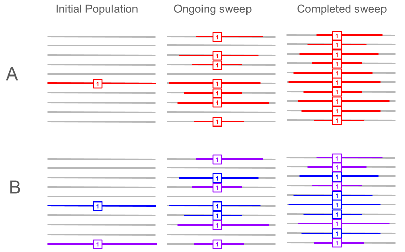
Figure 1. Schematic illustration of haplotype patterns under hard and soft selective sweeps. Panel (A) shows a hard sweep, where a single sweeping haplotype (red) rises from low frequency in the initial population (left column), to an ongoing sweep at ∼70% frequency (middle column), and ultimately to fixation at ∼100% frequency (right column), against a linked haplotype background (gray). Panel (B) shows a soft sweep, where selection acts on multiple haplotype backgrounds (blue and purple), which increase in frequency from the initial population (left column), to ∼70% during the ongoing sweep (middle column), and to near fixation/fixation in the final population (right column), while background haplotypes (gray) are reduced.
For incomplete sweeps where the selected allele is segregating at intermediate-tohigh frequency, single-population statistics such as iHS or nSL can be used and do not require a reference population when sample size is large enough. An incomplete sweep with the selected allele at ≈70% frequency can be detected using iHS/nSL in a sample of 10 diploid individuals. However, if sampling is reduced, within-population haplotype homozygosity estimates become noisier and iHS/nSL signals may weaken; in such cases, if a suitable reference population is available, XP-based comparisons (XP-EHH/XP-nSL) may retain greater power. In addition, for completed or near-completed sweeps (selected allele fixed or nearly fixed), iHS and nSL lose power and may become undefined because the locus may no longer be polymorphic in the sample. In this case, there will be few if any haplotypes lacking the adaptive allele to compare against. Therefore, cross-population methods (XP-EHH or XP-nSL) should improve power whenever a reference population exists.
Sweep type also affects method choice: hard sweeps typically generate a single dominant long haplotype and are relatively straightforward to detect with iHS/nSL, whereas soft sweeps involve multiple sweeping haplotype backgrounds and may not produce a single extreme haplotype, reducing sensitivity of iHS/nSL. In such cases, iHH12 provides a useful complement because it integrates EHH after combining the two most frequent haplotypes, improving sensitivity to sweeps occurring on multiple backgrounds; as illustrated in Figure 1, when haplotypes from both backgrounds (e.g., the blue and purple haplotypes) rise to high frequency, neither produces a uniquely dominant long-haplotype signal, and iHS/nSL for the derived allele will therefore be weaker. This occurs because extended haplotype homozygosity is effectively split across distinct sweeping backgrounds: in iHS each background is evaluated separately, and because the blue and purple haplotypes are not treated as the same haplotype, the EHH signal is reduced relative to a hard sweep where one dominant haplotype drives the signal.
When phasing is unavailable or uncertain, unphased implementations can be used, which is particularly relevant for non-model organisms; however, unphased methods generally require larger sample sizes to maintain power because heterozygous genotypes are effectively not used in the construction of unphased representations, reducing the amount of informative data contributing to the statistic.
Genetic map quality affects the reliability of statistics that integrate EHH over genetic distance, i.e., iHS and XP-EHH. When a dense and accurate recombination map is available, these methods can leverage genetic distance to account for local recombination-rate variation. However, in non-model organisms genetic maps might not be available and, when available, are often sparse or heavily interpolated, while recombination-rate variation can be extreme. These issues can distort integration distances (e.g., producing artificially short or collapsed genetic intervals) and increase missing values. In such cases, nSL and XP-nSL can be used as they are less sensitive to map artifacts and recombination-map uncertainty.
For readers interested in exploring the detailed effects of sample size, SNP density, recombination-rate variation, demography and other factors on the power and reliability of these haplotype-based statistics, we suggest consulting the original papers introducing iHS [19], nSL [20], iHH12 [30], XP-EHH [21], XP-nSL [22], and their unphased versions [24]. For example, [20] specifically addresses the effect of recombination rate variation, showing that iHS is more sensitive to local differences in recombination rate, whereas nSL remains comparatively robust under such conditions. It also demonstrates effect of demographic effects such as bottlenecks or expansion in population size.
Finally, several studies have shown that the correlation between iHS and nSL is often modest [33], suggesting that these statistics are powered in different regions of parameter space and capture complementary aspects of haplotype structure. This observation has motivated composite approaches, which integrate multiple selection statistics to improve robustness and localization power [36, 34]. More generally, because summary statistics vary in informativeness across selective and demographic scenarios, combining them improves reliability; this has been pursued using probabilistic frameworks that model dependencies among statistics (e.g., averaged one-dependence estimators [15]) as well as convolutional neural networks that learn patterns directly from summary statistic representations [14].
Overall, low correlation among statistics implies that they often highlight different candidate regions; therefore, relying on a single extreme outlier can be misleading, and candidate regions are best prioritized when supported by multiple complementary signals.
Two simple demographic history models, a single population model and a two population divergence model, were simulated to illustrate how the EHH-based statistics implemented in
In the single population model, the effective population size was set to Ne = 10,000, and, after a 100, 000 generation burn-in, a beneficial mutation (s = 0.1) was introduced at position 5 Mb in the 100, 001st generation. The simulation ran for an additional 2, 000 generations until the beneficial mutation reached ∼ 75% frequency. If the beneficial mutation was lost or did not reach ∼ 75% frequency, the simulation was restarted at the 100, 001st generation. At the end of a successful simulation, a VCF file was output. For the scenario with background selection deleterious mutations was introduced at a rate of 9 : 1, neutral:deleterious, with selection coefficients drawn from a gamma distribution with mean 0.1 and shape 0.2. Data for normalization was generated in the same way but without introducing a beneficial allele. 100 neutral replicates were generated for each scenario (with and without background selection). The neutral replicates were used to normalize the replicate containing the selected allele. Fifty individuals were sampled for each simulation. The resulting variants were filtered for biallelic SNPs and removed if the minor allele frequency below 0.05.
In the two population model, an ancestral population with effective population size Ne = 10,000 was simulated for a 100, 000 generation burn-in. At generation 100, 500, the ancestral population split into two populations each with effective population size Ne = 10,000. At generation 102, 000, a beneficial mutation (s = 0.1) was introduced into one population at position 5 Mb. The simulation ran for an additional 2, 000 generations until the beneficial mutation reached ∼ 75% frequency. If the beneficial mutation was lost or did not reach ∼ 75% frequency, the simulation was restarted at the 100, 001st generation. At the end of a successful simulation, a VCF file was output. For the scenario with background selection deleterious mutations was introduced at a rate of 9 : 1, neutral:deleterious, with selection coefficients drawn from a gamma distribution with mean 0.1 and shape 0.2. Data for normalization was generated in the same way but without introducing a beneficial allele. For each scenario, 100 neutral replicates were generated (with and without background selection). The neutral replicates were used to normalize the replicate containing the selected allele. Fifty individuals were sampled for each simulation. The resulting variants were filtered for biallelic SNPs.
For the two population model, with and without background selection, we investigated the effects of uneven sample sizes between the two populations. We tested sampling ten individuals from the first population and fifty individuals from the second population, and we tested sampling fifty individuals from the first population and ten individuals from the second population. This was done for the replicates containing the sweep as well as all neutral replicates. For each scenario, the resulting neutral replicates were used to normalize the replicate containing the sweep.
The phased and imputed genomes of two populations from the 1000 Genomes Project were used: 99 Utah individuals with Northern and Western European ancestry (CEU) and 108 Yoruba individuals from Ibadan, Nigeria (YRI) [41, 42]. All autosomes were extracted and were restricted to biallelic SNPs. For iHS, nSL, and iHH12 calculations,
Gene annotations were obtained from the GENCODE database (GRCh38) using the GTF file from [43].
In this section, we summarize the outcomes of applying
Figures 2 and 3 illustrate the importance of normalization for iHS and nSL. In Figures 2a and 3a, the raw statistic from the replicate containing the hard sweep is plotted against derived allele frequency, showing a clear correlation. This is because iHS and nSL are log-ratios of EHHc (Equation 3), which is summarizing haplotype lengths surrounding either the ancestral or derived alleles. As low-frequency alleles are likely to be younger and therefore segregate on longer haplotypes, even under neutrality, this implies larger log-ratio scores for low frequency alleles. Figures 2b and 3b show how normalization in frequency bins (Equation 14) corrects for this frequency bias. To underscore the importance of normalization, Figures 2c and 3c contrast raw |scores| and normalized |scores| as a function of genome location for the sweep simulation, clearly demonstrating that without normalization the sweep signal would be lost.
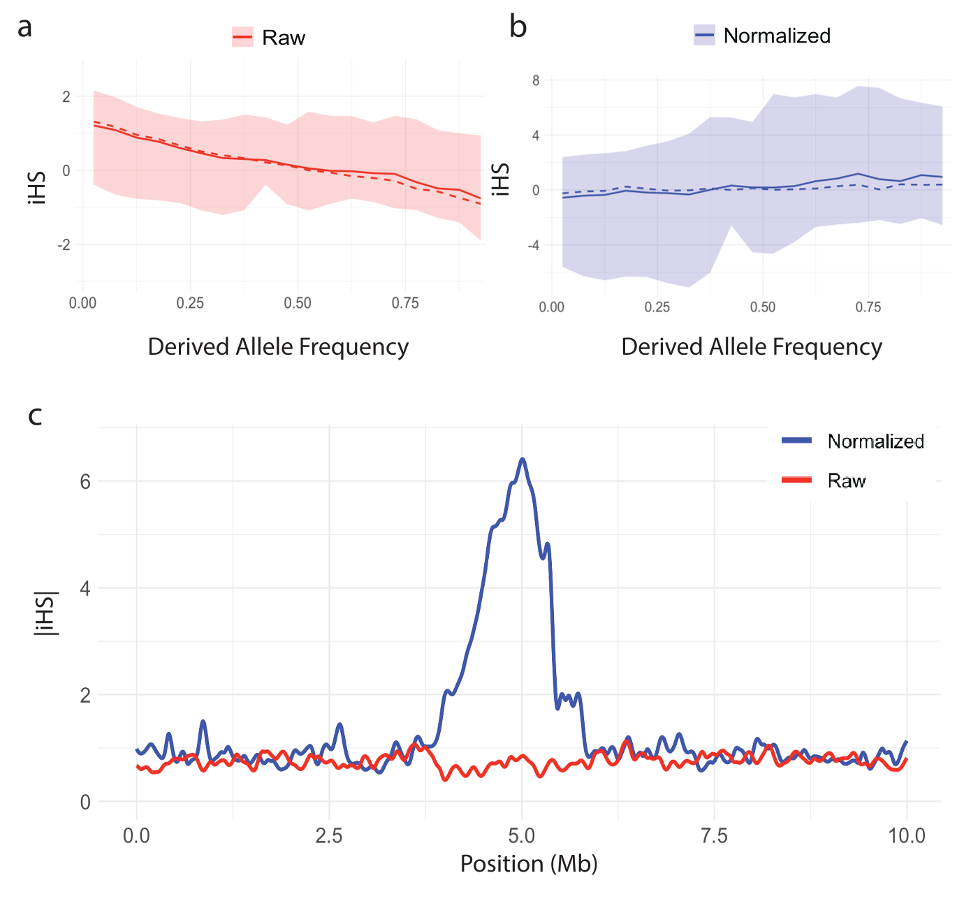
Figure 2. Distribution of the iHS statistic versus derived allele frequency and the effect of normalization. The mean (solid line), median (dashed line), and 1st-99th percentile range (shaded region) for (a) raw iHS and (b) normalized iHS statistic plotted against derived allele frequency. (c) Spline smoothed raw and normalized curves of |iHS| in the vicinity of a simulated hard sweep at 5Mb.
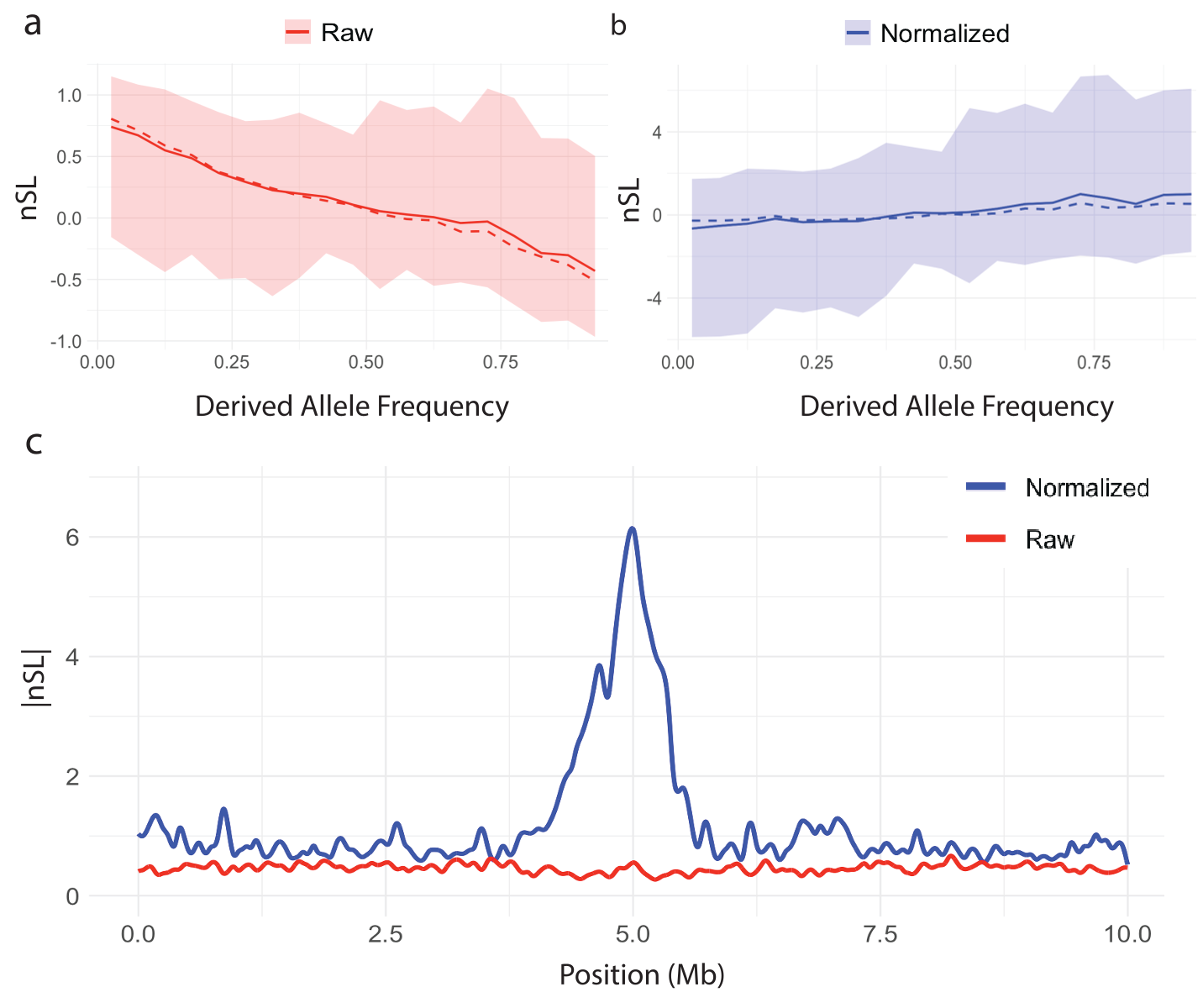
Figure 3. Distribution of the nSL statistic versus derived allele frequency and the effect of normalization. The mean (solid line), median (dashed line), and 1st-99th percentile range (shaded region) for (a) raw nSL and (b) normalized nSL statistic plotted against derived allele frequency. (c) Spline smoothed raw and normalized curves of |nSL| in the vicinity of a simulated hard sweep at 5Mb.
XPEHH and XPnSL, however, do not suffer from this dependence on derived allele frequency, as they are comprised of the EHH (Equation 1) of all haplotypes within each population, instead of restricting to haplotypes carrying a particular allele. This is illustrated in Figure 4. We show similar behavior for iHH12 in Figure 5. However, normalization is still recommended, as it puts different experiments on the same scale and allows for easy downstream statistical analyses which may assume variables are distributed Normally. We emphasize the that two-population statistic normalization does not depend on frequency (Equation 15) unlike single-population statistics.
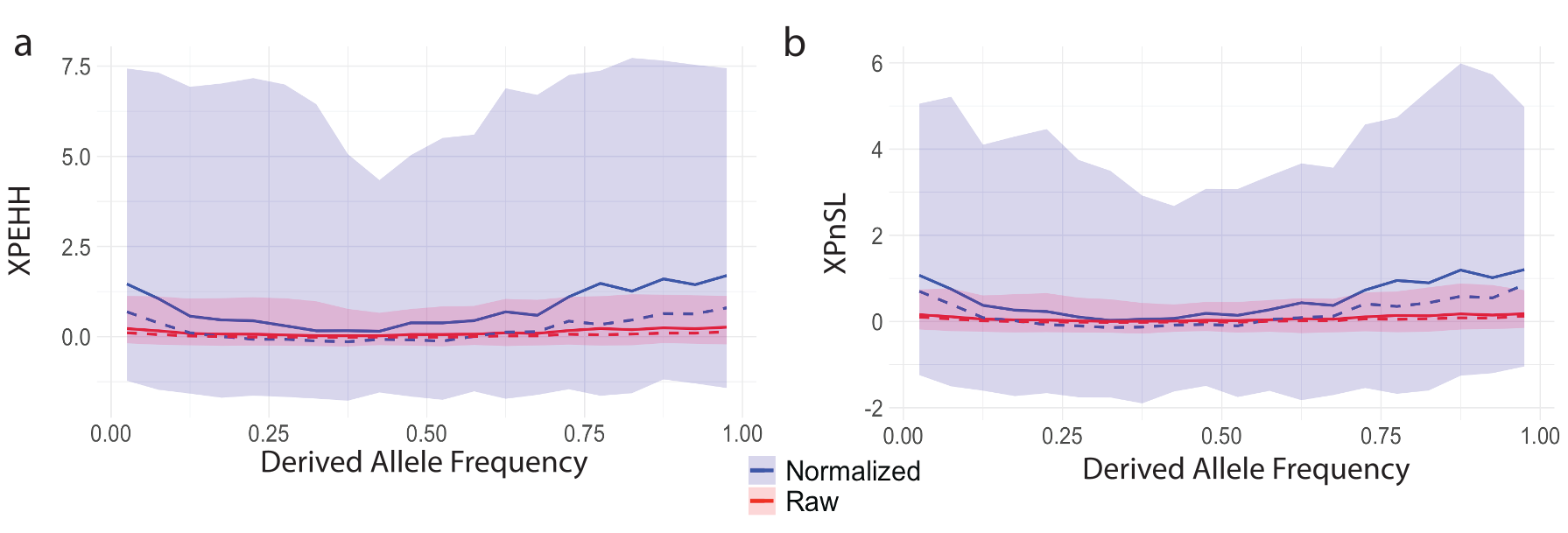
Figure 4. Distribution of cross-population statistics versus derived allele frequency. The mean (solid line), median (dashed line), and 1st-99th percentile range (shaded region) for (a) raw (red) and normalized (blue) XPEHH and (b) raw (red) and normalized (blue) XPnSL statistics plotted against derived allele frequency.
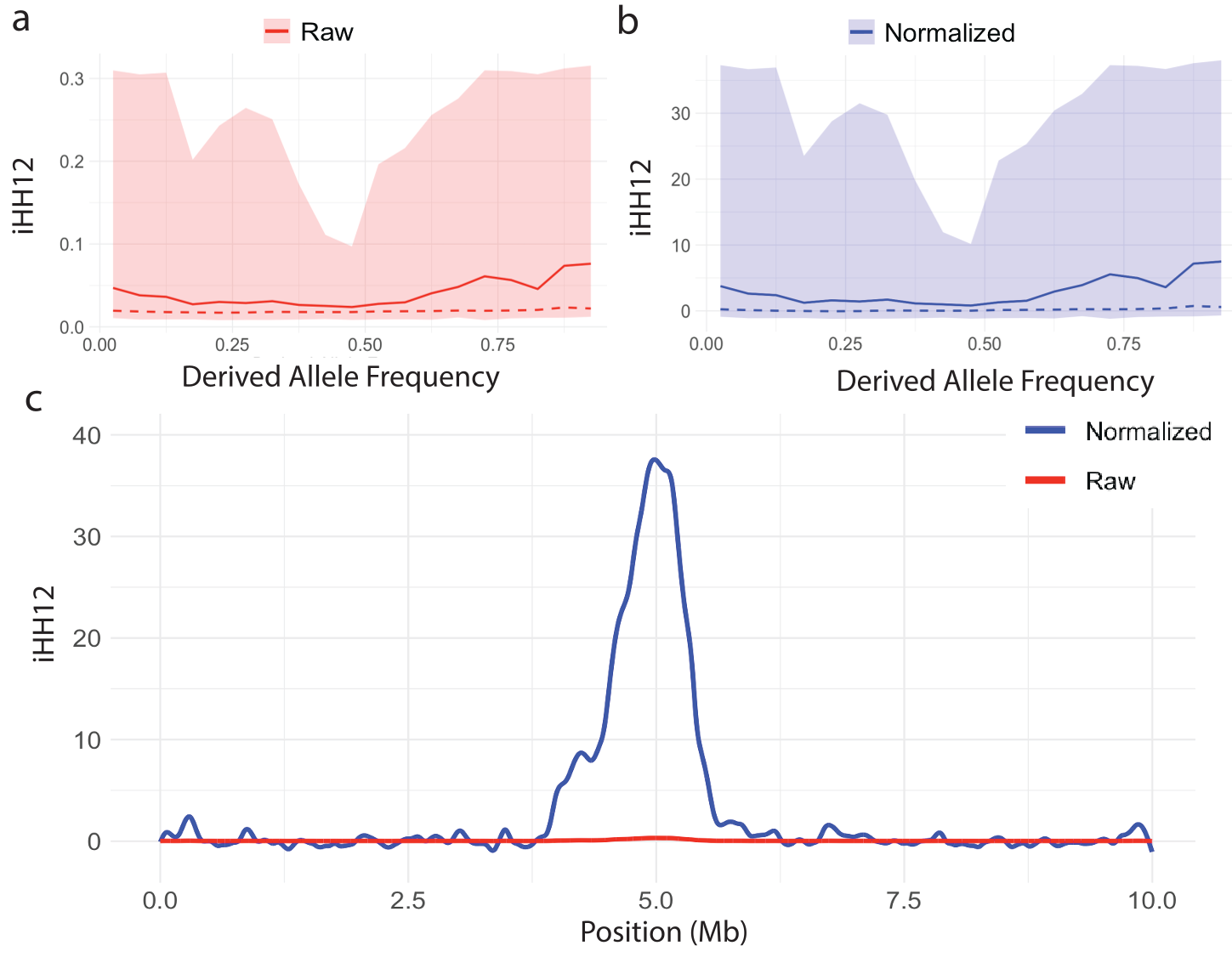
Figure 5. Distribution of the iHH12 statistic versus derived allele frequency and the effect of normalization. The mean (solid line), median (dashed line), and 1st-99th percentile range (shaded region) for (a) raw iHH12 and (b) normalized iHH12 statistic plotted against derived allele frequency. (c) Spline smoothed raw and normalized curves of |iHH12| in the vicinity of a simulated hard sweep at 5Mb.
Figure 6 illustrates how EHH can distinguish between genome regions with an adaptive allele sweeping and genome regions without an adaptive allele. Figure 6a plots the EHH of the entire sample in the vicinity of a sweep (dotted line), which decays slowly over distance, in contrast to the EHH in a neutral region (solid line) which decays quickly. Figure 6b illustrates how computing EHHc can distinguish between the sweeping haplotype and the non sweeping haplotype. In the sweep simulation, EHH1 is computed among the haplotypes carrying the adaptive derived allele, and haplotype homozygosity decays slowly. However, in the same simulation at the same locus, EHH0 is computed among the haplotypes not carrying the adaptive allele, and haplotype homozygosity decays quickly. Whereas in the neutral simulation both EHH1 and EHH0 decay quickly as neither set of hapotypes contain an adaptive allele. Figures 6c and 6d show similar patterns in the context of background selection. Based on these patterns, iHH12, iHS, and nSL are designed to efficiently summarize the contrasts in these curves for large-scale querying of millions of loci across a genome.
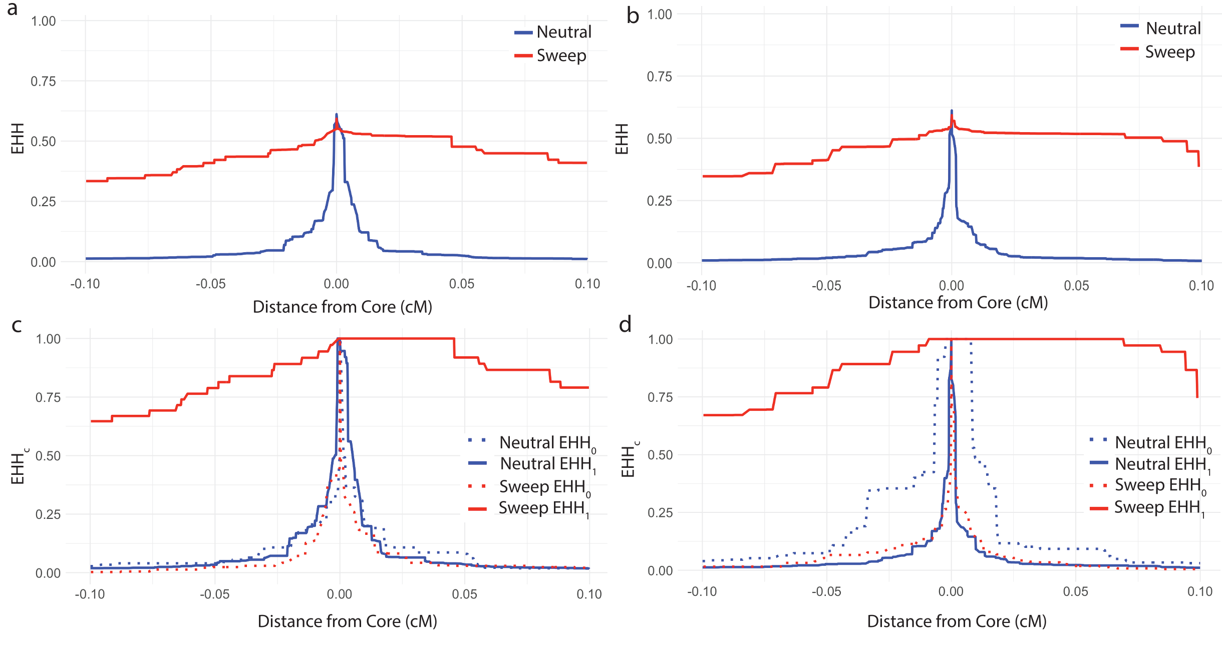
Figure 6. EHH and EHHc curves under different evolutionary scenarios. (a) EHH curves for a simulated hard sweep and a simulated neutral region. (b) EHHc curves for each of the core haplotypes (0 and 1) for a simulated hard sweep and a simulated neutral region. (c) EHH curves for a simulated hard sweep and a simulated region without a sweep in the presence of background selection. (d) EHHc curves for each of the core haplotypes (0 and 1) for a simulated hard sweep and a simulated region without a sweep in the presence of background selection.
Figure 7 illustrates how iHH12 (Figure 7a), iHS (Figure 7b), and nSL (Figure 7c) can identify a sweep in the center of a simulated 10Mb region. For all three statistics, regardless of the presence of background selection and regardless of whether allele phase is utilized (iHS and nSL only), a clear peak forms in the vicinity of where the adaptive allele was placed. This suggests that the EHH-based single-population statistics are robust to background selection.
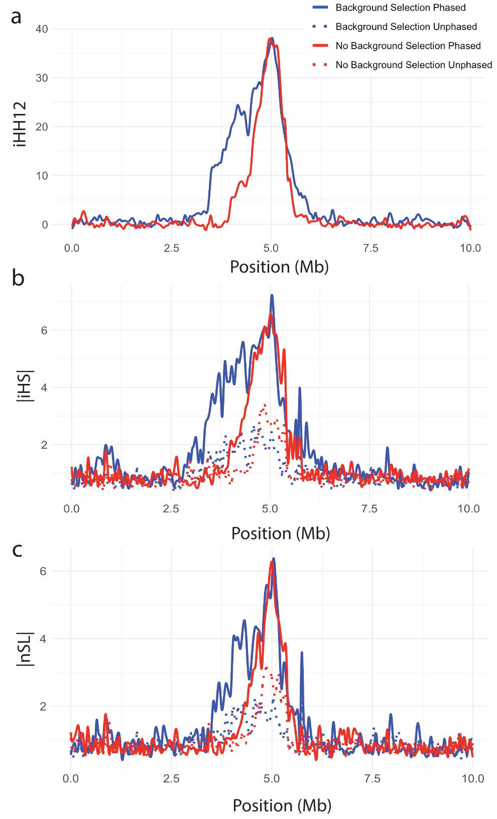
Figure 7. Single-population selection statistics showing clear sweep peaks. (a) iHH12, (b) |iHS|, and (c) |nSL| plotted against genomic position for a simulated hard sweep with and without background selection. All curves are splined smoothed.
The two-population statistics XPEHH and XPnSL are designed to summarize and contrast EHH patterns between two closely related populations to identify local adaptation. Figure 8 illustrates how these two statistics peak in the center of the simulated region where the adaptive allele was place. Figures 8a plot XPnSL and Figures 8b plot XPEHH. In addition to testing the influence of phased genotypes and background selection, the influence of unequal sample sizes among the two populations was considered, showing minimal influence Figure 9. This suggests that the EHH-based two-population statistics are robust to background selection and uneven samples size.
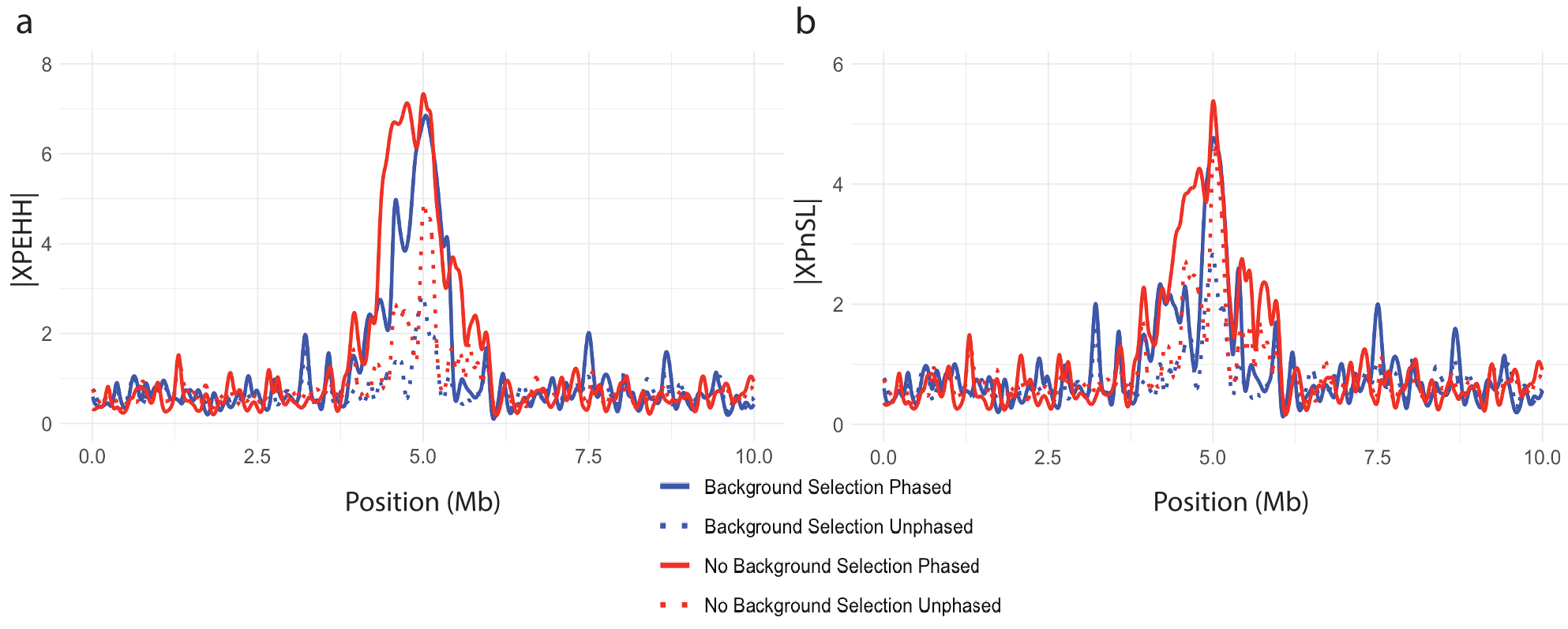
Figure 8. Cross-population selection statistics showing clear sweep peaks. Normalized (a) XPEHH and (b) XPnSL plotted against genomic position for a simulated hard sweep with and without background selection. All curves are splined smoothed.
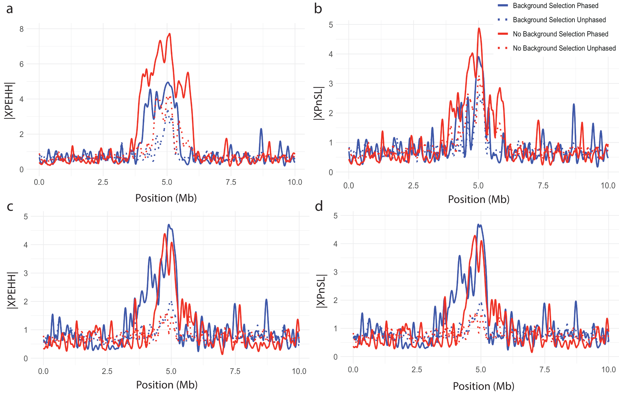
Figure 9. Effect of unequal sample sizes on cross-population statistics. Normalized (a) XPEHH with 50 sample from P1 and 10 samples from P2 (b) XPnSL with 50 sample from P1 and 10 samples from P2 (c) XPEHH with 10 sample from P1 and 50 samples from P2 (d) XPnSL with 10 sample from P1 and 50 samples from P2. All are plotted against genomic position for a simulated hard sweep with and without background selection. All curves are splined smoothed.
Section 3.1 demonstrates how
This section illustrates an example of
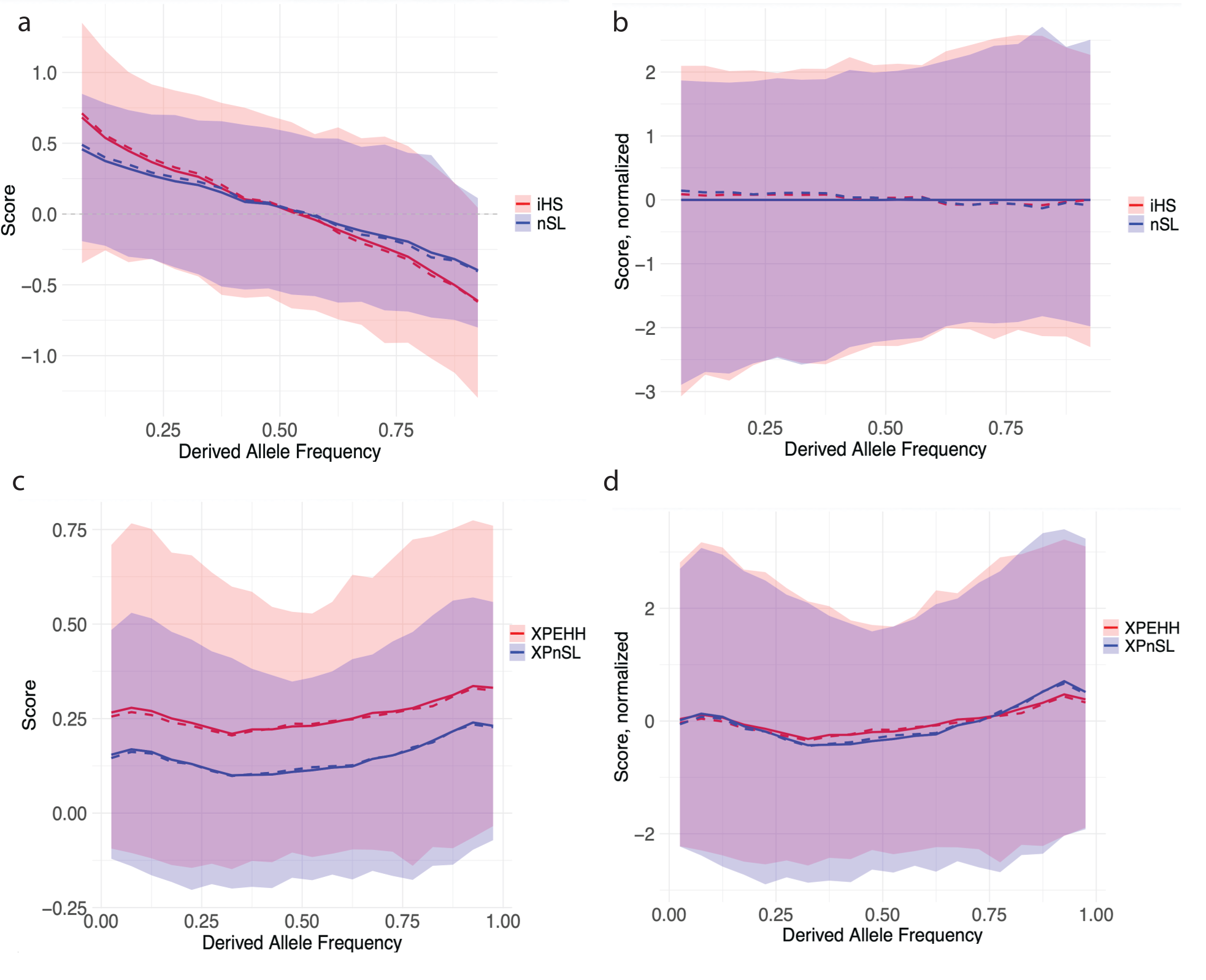
Figure 10. Distribution of EHH-based statistics versus derived allele frequency (DAF). (a) raw iHS (red) and nSL (blue) scores; (b) normalized iHS (red) and nSL (blue) scores; (c) raw XPEHH (red) and XPnSL (blue) scores; (d) normalized XPEHH (red) and XPnSL (blue) scores. All panels show the mean (solid line), median (dashed line), and 1st-99th percentile range (shaded area).
Focusing on chromosome 2 XPEHH scores,
Table 1. Top 20 windows on chromosome 2 from the top 1% of XP-EHH scores (sorted by maximum score column) showing the maximum score per window and the genes overlapping each window.
Zooming into the LCT/MCM6 locus, Figure 11a plots normalized |iHS| as a function of genome position on chromosome 2, and Figure 11b plots normalized XPEHH scores, as a function of genome position on chromosome 2. Both plots show broad peaks overlapping the LCT/MCM6, suggesting a clear signal of positive selection at this locus.
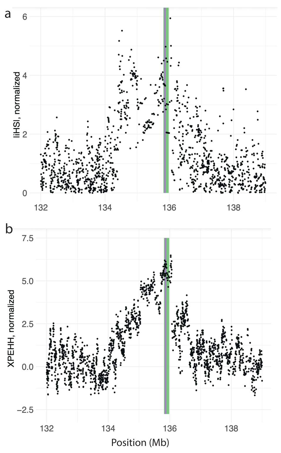
Figure 11. Two different selection statistics showing clear peaks overlapping the LCT/MCM6 region on chromosome 2 in CEU. Normalized (a) |iHS| plotted against chromosome 2 position in CEU, and normalized (b) XPEHH between CEU and YRI plotted against chromosome 2 position. The green shaded area highlights LCT, and the purple shaded area highlights MCM6.
Table 2. The table shows gene-level output from chromosome 2 for the CEU vs YRI comparison. Normalized XP-EHH scores were computed at the SNP level and standardized using the distribution across all autosomes. For each gene, all SNPs falling within the gene boundaries were collected. SNPs with normalized XP-EHH values greater than 2 were considered critical, and the “Fraction of Critical SNPs” column reports the proportion of such SNPs within each gene. Gene-level statistics were computed, including the maximum score, defined as the highest normalized XP-EHH value among all SNPs within the gene boundaries, and the length-corrected maximum score, which adjusts this maximum based on the distribution of scores across all genes on all autosomes to account for gene length. LCT and the gene MCM6, which contains an enhancer region approximately 14 kb upstream of LCT that regulates lactase expression, emerged as the top candidates on chromosome 2. We report the top 20 highest-scoring genes ranked by their length-corrected maximum score.
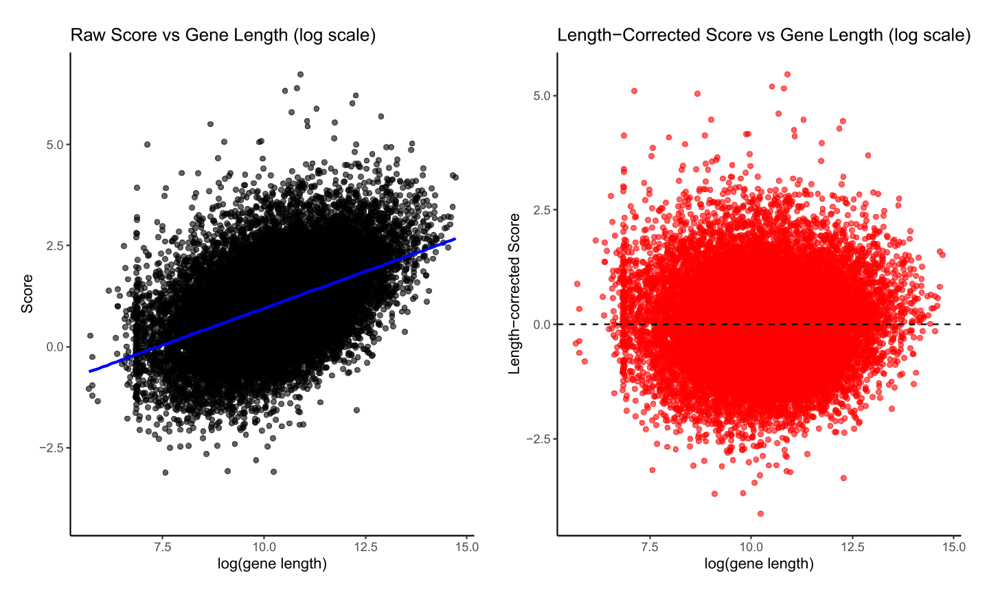
Figure 12. Length correction for XP-EHH scores in chromosome 2. Left panel: raw per-gene scores plotted against log(gene length), with a linear regression trend line (blue) showing the overall relationship. Right panel: length-corrected scores (residuals from the regression) plotted against logarithm of gene length, with a dashed line indicating the mean.
Figure 13 and Figure 14 compares selection signals across chromosome 2 for CEU. Each statistic operates in its own parameter space, and all detect the strong LCT-MCM6 signal, even without phase information. In our results, iHS and nSL (phased) show good correlation. At high SNP density (as in our data), these differences are small, but we can expect larger differences that break this correlation in other data where recombination rate varies, as discussed and experimentally shown in the original nSL paper. iHH12 captures soft sweeps and identifies more candidate regions overall, including rare, long haplotypes that iHS and nSL largely miss. The two unphased statistics are more similar to each other, as are the two phased statistics, while comparisons between phased and unphased versions show smaller correlation, reflecting slight information loss due to ignoring heterozygotes.
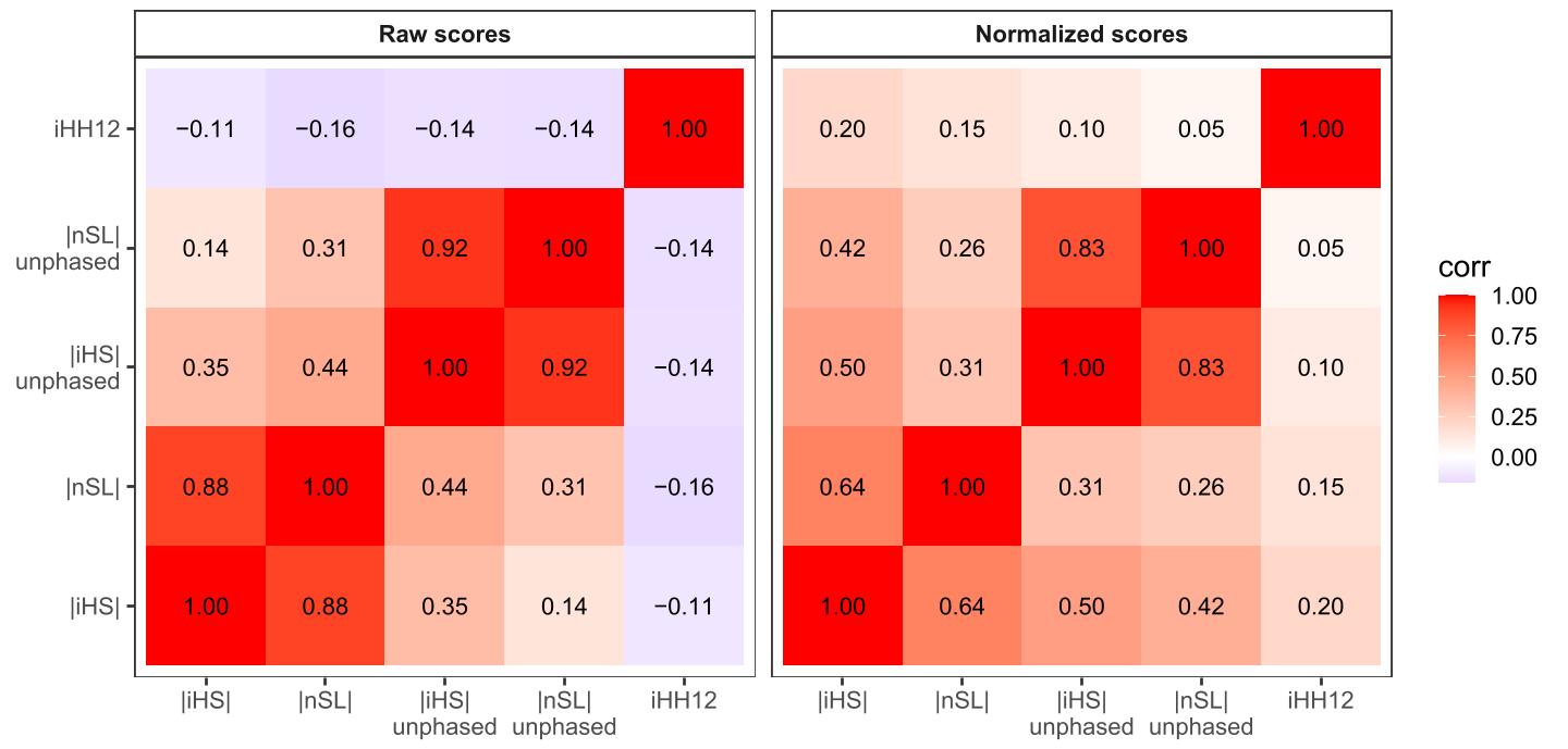
Figure 13. Pearson correlation of five selection statistics across chromosome 2 in the CEU population. Normalized scores (left panel) and raw scores (right panel) are shown for all single population statistics. Only positions where all statistics are defined are included. Values within tiles indicate the pairwise correlation.
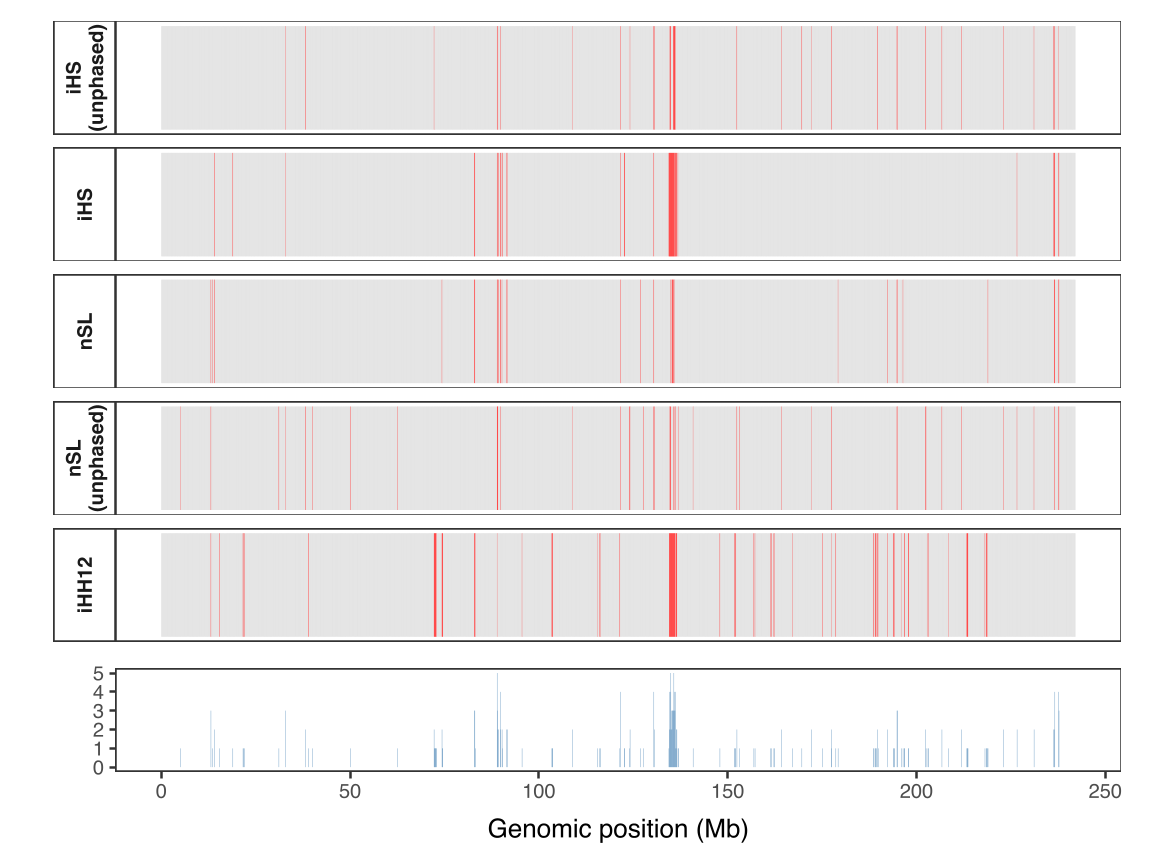
Figure 14. Comparison of aggregated selection scores (maximum per 100 kb window) across chromosome 2 in the CEU population. In the top panel, each tile represents a window for five statistics (iHS, nSL, iHS unphased, nSL unphased, iHH12), with red indicating windows in the top 1% and gray otherwise. The bottom panel shows the consensus score, indicating the number of statistics that are significant in each window (range 0-5). A peak in consensus is observed around the LCT-MCM6 region (≈135-136 Mb), reflecting strong concordance of high-scoring windows in this well-known lactose persistence locus. Only windows where all statistics are defined are included.
The use of selection statistics is ubiquitous in modern evolutionary genomics. The ability to identify putatively selected loci is of great importance in forming our understanding of adaptation of organisms to myriad selection pressures [2]. Therefore, the computation and analysis of selection statistics should be consistent across studies to maintain reproducibility of results and to ensure robust and reliable inference.
Many of the most widely used selection statistics for recombining genomes are based on Expected Haplotype Homozygosity (EHH), which measures the decay of haplotype identity away from a locus of interest [18, 21]. Here we provide the formal definition of EHH and the formal definitions of the EHH-based statistics iHS, nSL, iHH12, XPEHH, and XPnSL. All statistics and their unphased equivalents are implemented in the software
We demonstrated the use of
Ultimately, we hope to create a resource for the computation and interpretation of EHH-based selection statistics that is accessible to readers from various backgrounds. While
Not applicable.
Not applicable.
Computations for this research were performed using the Pennsylvania State University’s Institute for Computational Data Sciences’ Roar supercomputer. This work was supported by the National Institute of General Medical Sciences of the National Institutes of Health award number R35GM146926, and start-up funds from the Pennsylvania State University’s Department of Biology.
The authors have declared that no competing interests exist.
Conceptualization: A.R., T.Q.S., and Z.A.S.; Methodology: A.R. and T.Q.S.; Software: A.R.; Validation: A.R. and T.Q.S.; Formal Analysis: A.R. and T.Q.S; Investigation: A.R. and T.Q.S.; Resources: Z.A.S.; Data Curation: A.R. and T.Q.S.; Writing - Original Draft: A.R., T.Q.S., and Z.A.S.; Writing - Review & Editing: A.R., T.Q.S., and Z.A.S.; Visualization: A.R., T.Q.S., and Z.A.S.; Supervision: A.R. and Z.A.S.; Project Administration: Z.A.S.; Funding Acquisition: Z.A.S.
The authors would like to four anonymous reviewers for their helpful comments.
| 1. | Scheinfeldt LB, Tishkoff SA. Recent human adaptation: genomic approaches, interpretation and insights. Nat Rev Genet. 2013;14(10):692-702. [Google Scholar] [CrossRef] |
| 2. | Fu W, Akey JM. Selection and adaptation in the human genome. Annu Rev Genomics Hum Genet. 2013;14(1):467-489. [Google Scholar] [CrossRef] |
| 3. | Benton ML, Abraham A, LaBella AL, Abbot P, Rokas A, Capra JA. The influence of evolutionary history on human health and disease. Nat Rev Genet. 2021;22(5):269-283. [Google Scholar] [CrossRef] |
| 4. | Booker TR, Jackson BC, Keightley PD. Detecting positive selection in the genome. BMC Biol. 2017;15:98. [Google Scholar] [CrossRef] |
| 5. | Pavlidis P, Alachiotis N. A survey of methods and tools to detect recent and strong positive selection. J Biol Res Thessalon. 2017;24(1):7. [Google Scholar] [CrossRef] |
| 6. | Szpiech ZA, Hernandez RD. Selective sweeps. In: Encyclopedia of Evolutionary Biology. Oxford, UK: Elsevier Inc.; 2016. p. 23–32. |
| 7. | Nielsen R, Williamson S, Kim Y, Hubisz MJ, Clark AG, Bustamante C. Genomic scans for selective sweeps using snp data. Genome Res. 2005;15(11):1566-1575. [Google Scholar] [CrossRef] |
| 8. | DeGiorgio M, Huber CD, Hubisz MJ, Hellmann I, Nielsen R. Sweepfinder2: increased sensitivity, robustness and flexibility. Bioinformatics. 2016;32(12):1895-1897. [Google Scholar] [CrossRef] |
| 9. | Harris AM, DeGiorgio M. A likelihood approach for uncovering selective sweep signatures from haplotype data. Mol Biol Evol. 2020;37(10):3023-3046. [Google Scholar] [CrossRef] |
| 10. | DeGiorgio M, Szpiech ZA. A spatially aware likelihood test to detect sweeps from haplotype distributions. PLoS Genet. 2022;18(4):e1010134. [Google Scholar] [CrossRef] |
| 11. | Stern AJ, Wilton PR, Nielsen R. An approximate full-likelihood method for inferring selection and allele frequency trajectories from dna sequence data. PLoS Genet. 2019;15(9):e1008384. [Google Scholar] [CrossRef] |
| 12. | Vaughn AH, Nielsen R. Fast and accurate estimation of selection coefficients and allele histories from ancient and modern dna. Mol Biol Evol. 2024;41(8):msae156. [Google Scholar] [CrossRef] |
| 13. | Hejase HA, Mo Z, Campagna L, Siepel A. A deep-learning approach for inference of selective sweeps from the ancestral recombination graph. Mol Biol Evol. 2022;39(1):msab332. [Google Scholar] [CrossRef] |
| 14. | Kern AD, Schrider DR. diplos/hic: an updated approach to classifying selective sweeps. G3 (Bethesda). 2018;8(6):1959-1970. [Google Scholar] [CrossRef] |
| 15. | Sugden LA, Atkinson EG, Fischer AP, Rong S, Henn BM, Ramachandran S. Localization of adaptive variants in human genomes using averaged one-dependence estimation. Nat Commun. 2018;9(1):703. [Google Scholar] [CrossRef] |
| 16. | Amin MR, Hasan M, DeGiorgio M. Digital image processing to detect adaptive evolution. Mol Biol Evol. 2024;41(12):msae242. [Google Scholar] [CrossRef] |
| 17. | Arnab SP, Campelo dos Santos AL, Fumagalli M, DeGiorgio M. Efficient detection and characterization of targets of natural selection using transfer learning. Mol Biol Evol. 2025;42(5):msaf094. [Google Scholar] [CrossRef] |
| 18. | Sabeti PC, Reich DE, Higgins JM, Levine HZP, Richter DJ, Schaffner SF, et al. Detecting recent positive selection in the human genome from haplotype structure. Nature. 2002;419(6909):832-837. [Google Scholar] [CrossRef] |
| 19. | Voight BF, Kudaravalli S, Wen X, Pritchard JK. A map of recent positive selection in the human genome. PLoS Biol. 2006;4(3):e72. [Google Scholar] [CrossRef] |
| 20. | Ferrer-Admetlla A, Liang M, Korneliussen T, Nielsen R. On detecting incomplete soft or hard selective sweeps using haplotype structure. Mol Biol Evol. 2014;31(5):1275-1291. [Google Scholar] [CrossRef] |
| 21. | Sabeti PC, Varilly P, Fry B, Lohmueller J, Hostetter E, Cotsapas C, et al. Genome-wide detection and characterization of positive selection in human populations. Nature. 2007;449(7164):913-918. [Google Scholar] [CrossRef] |
| 22. | Szpiech ZA, Novak TE, Bailey NP, Stevison LS. Application of a novel haplotype-based scan for local adaptation to study high-altitude adaptation in rhesus macaques. Evol Lett. 2021;5(4):408-421. [Google Scholar] [CrossRef] |
| 23. | Klassmann A, Gautier M. Detecting selection using extended haplotype homozygosity (ehh)-based statistics in unphased or unpolarized data. PloS One. 2022;17(1):e0262024. [Google Scholar] [CrossRef] |
| 24. | Szpiech ZA. selscan 2.0: scanning for sweeps in unphased data. Bioinformatics. 2024;40(1):btae006. [Google Scholar] [CrossRef] |
| 25. | Szpiech ZA, Hernandez RD. selscan: an efficient multithreaded program to perform ehh-based scans for positive selection. Mol Biol Evol. 2014;31(10):2824-2827. [Google Scholar] [CrossRef] |
| 26. | Rahman A, Smith TQ, Szpiech ZA. Fast and memory-efficient dynamic programming approach for large-scale ehh-based selection scans. Mol Biol Evol. 2025;42(11):msaf275. [Google Scholar] [CrossRef] |
| 27. | Gautier M, Vitalis R. rehh: an r package to detect footprints of selection in genome-wide snp data from haplotype structure. Bioinformatics. 2012;28(8):1176-1177. [Google Scholar] [CrossRef] |
| 28. | Gautier M, Klassmann A, Vitalis R. rehh 2.0: a reimplementation of the r package rehh to detect positive selection from haplotype structure. Mol Ecol Resour. 2017;17(1):78-90. [Google Scholar] [CrossRef] |
| 29. | Maclean CA, Chue Hong NP, Prendergast JGD. Hapbin: an efficient program for performing haplotype-based scans for positive selection in large genomic datasets. Mol Biol Evol. 2015;32(11):3027-3029. [Google Scholar] [CrossRef] |
| 30. | Torres R, Szpiech ZA, Hernandez RD. Human demographic history has amplified the effects of background selection across the genome. PLoS Genet. 2018;14(6):1-27. [Google Scholar] [CrossRef] |
| 31. | Garud NR, Messer PW, Buzbas EO, Petrov DA. Recent selective sweeps in north american drosophila melanogaster show signatures of soft sweeps. PLoS Genet. 2015;11(2):1-32. [Google Scholar] [CrossRef] |
| 32. | Lopes I, Altab G, Raina P, de Magalhães JP. Gene size matters: An analysis of gene length in the human genome. Front Genet. 2021;12:559998. [Google Scholar] [CrossRef] |
| 33. | Ma Y, Ding X, Qanbari S, Weigend S, Zhang Q, Simianer H. Properties of different selection signature statistics and a new strategy for combining them. Heredity. 2015;115(5):426-436. [Google Scholar] [CrossRef] |
| 34. | Sajid Randhawa IA, Khatkar MS, Thomson PC, Raadsma HW. Composite selection signals can localize the trait specific genomic regions in multi-breed populations of cattle and sheep. BMC Genet. 2014;15(1):34. [Google Scholar] [CrossRef] |
| 35. | Gage JL, White MR, Edwards JW, Kaeppler S, de Leon N. Selection signatures underlying dramatic male inflorescence transformation during modern hybrid maize breeding. Genetics. 2018;210(3):1125-1138. [Google Scholar] [CrossRef] |
| 36. | Grossman SR, Andersen KG, Shlyakhter I, Tabrizi S, Winnicki S, Yen A, et al. Identifying recent adaptations in large-scale genomic data. Cell. 2013;152(4):703-713. [Google Scholar] [CrossRef] |
| 37. | Purcell S, Neale B, Todd-Brown K, Thomas L, Ferreira MAR, Bender D, et al. Plink: a tool set for whole-genome association and population-based linkage analyses. Am J Hum Genet. 2007;81(3):559-575. [Google Scholar] [CrossRef] |
| 38. | Baumdicker F, Bisschop G, Goldstein D, Gower G, Ragsdale AP, Tsambos G, et al. Efficient ancestry and mutation simulation with msprime 1.0. Genetics. 2022;220(3):iyab229. [Google Scholar] [CrossRef] |
| 39. | Howie BN, Donnelly P, Marchini J. A flexible and accurate genotype imputation method for the next generation of genome-wide association studies. PLoS Genet. 2009;5(6):e1000529. [Google Scholar] [CrossRef] |
| 40. | Haller BC, Ralph PL, Messer PW. Slim 5: Eco-evolutionary simulations across multiple chromosomes and full genomes. Mol Biol Evo. 2026;43(1):msaf313. [Google Scholar] [CrossRef] |
| 41. | 1000 Genomes Project Consortium, Auton A, Brooks LD, Durbin RM, Garrison EP, Kang HM, et al. A global reference for human genetic variation. Nature. 2015;526(7571):68-74. [Google Scholar] [CrossRef] |
| 42. | Byrska-Bishop M, Evani US, Zhao X, Basile AO, Abel HJ, Regier AA, et al. High-coverage whole-genome sequencing of the expanded 1000 genomes project cohort including 602 trios. Cell. 2022;185(18):3426-3440.e19. [Google Scholar] [CrossRef] |
| 43. | Frankish A, Diekhans M, Jungreis I, Lagarde J, Loveland JE, Mudge JM, et al. Gencode 2021. Nucleic Acids Res. 2021;49(D1):D916-D923. [Google Scholar] [CrossRef] |
| 44. | Tishkoff SA, Reed FA, Ranciaro A, Voight BF, Babbitt CC, Silverman JS, et al. Convergent adaptation of human lactase persistence in africa and europe. Nat Genet. 2007;39(1):31-40. [Google Scholar] [CrossRef] |
| 45. | Ingram CJE, Mulcare CA, Itan Y, Thomas MG, Swallow DM. Lactose digestion and the evolutionary genetics of lactase persistence. Hum Genet. 2009;124:579-591. [Google Scholar] [CrossRef] |
| 46. | Huber CD, DeGiorgio M, Hellmann I, Nielsen R. Detecting recent selective sweeps while controlling for mutation rate and background selection. Mol Ecol. 2016;25(1):142-156. [Google Scholar] [CrossRef] |

![]()
Copyright © 2026 Pivot Science Publications Corp. - unless otherwise stated | Terms and Conditions | Privacy Policy


